Experimental Clarification of Coulomb-Field Propagation
Superluminal information transfer confirmed by simple experiment
Wolfgang G. Gasser (May, 2016)
PDF Version – Kurze Version auf Deutsch
Abstract
A simple experiment has been performed in order to measure propagation speed of the electric field. The results show that the Coulomb interaction propagates substantially faster than at speed of light c.
Fig. 1: Schematic of the experiment
The experiment uses a spark gap between two conducting spheres acting as capacitors of opposite electric charge. After spark-formation, this rapidly collapsing dipole field is measured by an oscilloscope connected via probes to conducting detector-spheres. Whereas the mutual distance between the detector spheres connected to the oscilloscope remains at Δx = 1.65 m (from left probe tip to right probe tip), different distances from the spark-gap have been measured.
|
Id. |
x_left |
x_right |
Δx |
Δt |
v = Δx/Δt |
|
|
1.85 m |
3.5 m |
1.65 m |
3.3 ns |
1.7 c |
||
|
2.6 m |
4.25 m |
1.65 m |
1.1 ns |
5.0 c |
||
|
3.35 m |
5 m |
1.65 m |
1.7 ns |
3.2 c |
||
|
4.85 m |
6.5 m |
1.65 m |
2.1 ns |
2.6 c |
||
|
6.35 m |
8 m |
1.65 m |
2.9 ns |
1.9 c |
||
|
7.85 m |
9.5 m |
1.65 m |
3.8 ns |
1.5 c |
||
|
9.35 m |
11 m |
1.65 m |
4.0 ns |
1.4 c |
Tab. 1
The measured propagation speeds v = Δx/Δt from the left to the right detector sphere, with Δt averaged over each five measurements, range from around 1.4 c to 5 c, and show a dependence on the distance from the spark gap.
The by far simplest explanation of the experiment is the hypothesis that the Coulomb interaction conforms to Coulomb, who assumed instantaneous interaction at a distance. The dependence of the measured propagation speed on the distance of the measurement setup from the spark gap is explained by dissipative losses and "image charge" complication, leading to electric currents in the ground and the walls.
o Dipole field with and without mirror resp. image charges
o Tests and control experiment
o Possible improvements of the experiment
Before Heinrich Hertz succeeded 1887 in experimentally demonstrating the existence of electromagnetic waves propagating at c, he had already detected "an infinite rate of propagation in air". Hertz writes on his first attempts:
"But when I had carefully set up the apparatus and carried out the experiment, I found that the phase of the interference was obviously different at different distances, and that the alternation was such as would correspond to an infinite rate of propagation in air. Disheartened, I gave up experimenting." (See)
It is reasonable to assume that in trying to create longitudinal waves, Hertz had detected the Coulomb field of an electrically oscillating capacitor. As classical physics was based on instantaneous actions at a distance, and the then new Faraday-Maxwell electrodynamics was based on general propagation at c, Hertz considered his measurements of such timeless interactions simply as irrelevant and/or erroneous.
Since the very first experiments performed by Hertz, instantaneous actions at a distance have continued to haunt electromagnetism. As static interference measurements were the main tool to detect such effects, they could always be dismissed by the hypothesis that they are caused by systematic errors such as unwanted reflections.
With the advent of modern measurement equipment with clock cycles in the order of nanoseconds, the situation has dramatically changed. Unnoticed, it has become possible to easily measure the propagation speed of electric fields by direct time measurements.
The experiment, based on spark-triggered rapid collapse of an electric field, has been performed in a sports hall (concrete-steel construction). Because of the mirror-charge problem, the experiment has been performed at a height of 2 m above ground. The mirror image of the emitter-dipole due to the (steel in) ground is thus about 4 m below the actual dipole.
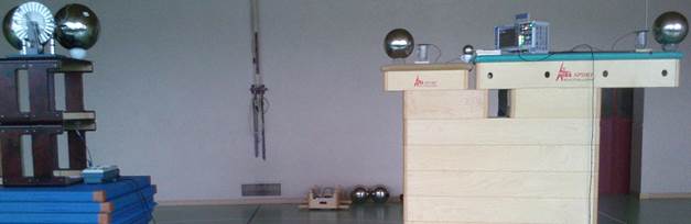
The emitter on the left consists of two metallic spheres forming a spark gap. In order to charge the dipole-spheres, a Wimshurst influence machine is used. As the spheres are used as high-voltage capacitors, the capacitor of the influence machine has been disconnected.
The measurement setup on the right of the photo contains the (main) oscilloscope and two (main) detector spheres, which are connected to the oscilloscope. One probe is connected to right side of the left (nearby) detector-sphere, and a second probe to left side of right (remote) sphere. The distance Δx between the probe-tips is 1.65 m (and 2.15 m between the outsides of the detector spheres with each a diameter of 0.25 m).
Charging the dipole on the left takes typically a few seconds until electric breakdown. During this charging period, voltages in the measurement setup change slowly, and are compensated by negligible currents through the probes connecting the detector spheres with the oscilloscope.
The spark gap is several millimeters, and the spheres are charged to in the order of +5000 and -5000 Volt. Spark breakdown leads to a continuous conducting channel between the spheres, and the dipole starts rapidly to discharge.
It is the start of the discharge which is used as a "single-shot" event in order to determine the speed of the propagation of the electric field. Thus, not only the distinction between group and phase velocity becomes irrelevant, but also the subsequently emerging complex oscillations (oscillations within one sphere, through the spark gap, through the oscilloscope, of whole sports hall; generation, absorption and reflection of transversal radiation).
The experiment deals with the propagation time Δt of the discharge signal from the left to right detector sphere. Ideally, the hypothesis of Coulomb would result in Δt = 0, and the hypothesis of Maxwell and Special Relativity in Δt = Δx / c = 5.5 ns.
Let us assume that at t = 0, a relevant field decrease from the dipole has reached the left detector-sphere up to the probe-tip (see Fig. 1). The Coulomb force accumulating electrons on the left detector sphere has therefore become lower. As the repulsion between the electrons on this spherical capacitor is no longer fully compensated by the dipole, electrons start to get pushed from this capacitor via the probe into the oscilloscope. This electron flow shows up as a negative voltage-signal on the oscilloscope. The decrease of the dipole-field having reached the left probe-tip at t = 0 is assumed by modern physics to reach the right detector-sphere only at t = 1.65 m / c = 5.5 ns. Any signal from the right probe, depending on the presence of the right (remote) sphere, should be retarded by at least 5.5 ns with respect to the left signal.
Changes of the Coulomb field caused by the spark strongly decrease with distance (see below). Therefore, dissipative losses entail that for a field change detectable at the remote detector sphere, the dipole must discharge longer than for detectability at the nearby sphere.
For results see Tab. 1. The spreadsheet calculations (with links to the original data) can be found here.
Dipole field with and without mirror resp. image charges
The charge distribution of such a dipole consisting of two spherical capacitors is quite complicated. The dipole of the experiment consists of two metallic spheres with each a radius of 17.5 cm. As charge density is highest near the spark gap (due to mutual attraction), let us use a simplification in order to explain the principle of the experiment:
An ideal dipole consists of two point charges with -q0 at position x = –0.15 m and +q0 at position x = 0.15 m, where q0 = 8.34 x 10⁻⁸ Coulomb (around 5.2 x 10¹¹ elementary charges). At a distance of 0.15 m from such a point charge q0, the potential (with respect to infinity) is 5000 V. This also means that if a conducting sphere with radius 0.15 m has charge q0, then its surface voltage is 5000 V.
The blue line of Fig. 2a shows the electric field in Volt per meter caused by the dipole up to a distance of 10 m on our measurement line resp. dipole axis 2 m above ground.
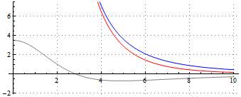
Fig. 2a: Horizontal axis: distance in meter; vertical axis: electric field in V/m
Now let us assume a conducting plane 2 m below the dipole axis. The dipole above the ground leads to a charge distribution on the ground, compensating for the electric field resp. voltage created by the dipole. This charge distribution on the ground can be derived from a hypothetical charge-inverted image of the dipole mirrored by the ground. This hypothetical image dipole 4 m below the real dipole creates on our measurement line (in direction of the dipole axis) an electric field which apart from the region close to the dipole has opposite sign of the field created by the real dipole. The gray line of Fig. 2a shows the electric field created by the image dipole on and in direction of our measurement line, and the red line the total field created by both real dipole and image-dipole.
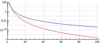
Fig. 2b: Horizontal axis: distance in meter; vertical axis: electric field in V/m
Fig. 2b with logarithmic scale shows that far enough from the dipole, the total field (i.e. together with field from the image dipole) decreases substantially more with distance than the field from the real dipole alone. Whereas at far enough distances, the field of the real dipole decreases in proportion to r-3, the total field decreases in proportion to r-5.
The strong decrease can easily be understood. Let us take a distance of 100 m from the dipole. As the image dipole is 4 m below our measurement line resp. dipole axis, its distance remains with r = √[1002+42] m = 100.08 m close to 100 m. Also the angle with respect to our measurement-line is rather small. As the image dipole is inversely charged, it cancels a substantial part of the field created by the real dipole.
This decrease in proportion to r-5 due to image charges is a main reason for the difficulty to use changing Coulomb-dipole fields in order to transmit signals in longitudinal direction over relevant distances.
A further problem arises. Together with the discharging dipole, the reason for the mirror-charge distribution on the ground (and/or elsewhere) disappears, and the electrons of the ground responsible for this mirror-charge distribution start to move back. This problem is especially acute, if the ground is a good conductor (e.g. because it contains reinforcing steel).
Fig. 3 shows the potential created by the image dipole on the ground just under our measurement line (i.e. under the dipole axis being 2 m above ground). (Parameters: above presented illustration values):
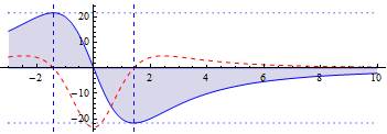
Fig. 3: Horizontal axis: distance in meter from dipole; vertical axis: electric potential due to "image" charge distribution on the ground in Volt; red dashed line: electric field in V/m
This electric potential due to the image dipole is the exact opposite of the potential created by the real dipole. So whereas at xminV = 1.42 m (the right of the vertical blue dashed lines) the real dipole is responsible for the maximal voltage of 21.6 Volt, the hypothetical image dipole compensates this with exactly –21.6 Volt. In this way, the (electrically grounded) ground remains electrically neutral.
The "image-dipole" voltage is in reality created by a concrete charge distribution on the ground. The electric field caused by these charges on the ground in measurement direction is shown in Fig. 3 by the red dashed line.
For simplicity, let us assume that the real dipole fully disappears during a negligible time interval. Then the negative charge distribution on the ground under the right dipole-side is no longer compensated by the dipole-field, and the electrons on the ground immediately start to move back. At x > xminV = 1.42 m the electric field is positive, and the electrons start to move to the right. Only between the two blue dashed lines of Fig. 3, i.e. from around x = -1.42 m to x = +1.42 m, the electric field is negative and electrons start to move to the left. The field change of such an electron bulge moving (maximally) at around v = 2/3 c rightwards toward a detector sphere causes there a field change in the same direction as the one caused by the discharging dipole.
An ideal electron bulge moving at v = 2/3 c on the ground rightwards to the measurement setup would at first show up as a negative signal of the left detector sphere, as the electrons of this sphere are repelled by the approximating electron bulge, and are therefore pushed into the oscilloscope. Only Δt = Δx / v = 8.2 ns later, the electron bulge reaches the distance necessary for having a comparable effect on the right detector sphere. This time, the electrons of the right detector sphere are repelled away from the oscilloscope, leading to a positive signal (i.e. inverted and retarded by 8.2 ns with respect to the signal from the left detector sphere.)
The effect of such moving charges (i.e. currents) on or in the ground or walls must not be confused with the direct effect from the dipole.
Grounding (earthing)
The short grounding wires belonging to the probes have been removed. Thus the core of the probe cable is the only input into the oscilloscope. This constitutes no problem: If we touch with a probe an isolated detector sphere having been charged previously to 6 Volt, then a sharp slope to 6 Volt shows up on the oscilloscope. At 6 Volt the charge of a sphere with radius r = 12.5 cm is q = 4.34 x 10⁻¹¹ C (because q / (4πε0 r) = 6 Volt). The probe has a resistance of 1 MOhm. Thus the sphere starts to discharge via the probe at a current of 6 μA, i.e. 6 x 10-15 Coulomb per nanosecond.
Grounding of the oscilloscope affects the end of the first signal-slope caused by the collapsing emitter-dipole field, but has no relevant effect on the start of the signal.
The oscilloscope has been grounded via the grounding line of the power cord. In order to minimize disturbances coming from the power cord, a long extension cable has been used and placed in such a way next to oscilloscope, that the first meters connected to oscilloscope could not be relevantly disturbed by the strong field changes caused by the dipole-sparks.
If such a measurement setup is completely isolated, then the nearby detector sphere becomes negatively and the remote detector sphere positively charged during charging the emitter dipole. The electron surplus of the nearby left detector sphere essentially stems from the remote one.
![]()
Fig. 4a: Charge distribution of an isolated measurement setup
The whole measurement setup (oscilloscope and detector spheres) is then at a same positive potential, as no charge from outside can compensate for the positive potential created by the dipole.
If the oscilloscope is grounded, then the whole measurement setup becomes negatively charged.
![]()
Fig. 4b: Charge distribution of a grounded measurement setup
The induced negative charges compensate for the positive potential resp. voltage created by the dipole, with the result that the whole measurement setup is at total potential zero (potential of the ground).
When the dipole field collapses after spark formation, the charge distribution of the measurement setup of Fig. 4b is no longer compensated by an external field. The remote (right) detector sphere, despite being negatively charged, is less negative than the oscilloscope. So, the sphere as a capacitor starts sucking in electrons from the oscilloscope, showing up as positive voltage signal on the screen. In the end however, both the negative charge of nearby detector sphere and the smaller negative charge of the remote detector sphere will flow away via the grounding connection of the oscilloscope. Thus, both channels end up showing negative voltages, until the spheres are discharged via the 1 Mega-Ohm probes.
Fig. 5a/5b: Further development of input signals after spark formation (50 ns/div in 5a, 500 ns/div in 5b)
In Fig. 5 (from config_c) one can see that the signal from the remote detector sphere at first goes upward, but after strong oscillations stabilizes at around –1.7 Volt. The signal from the left nearby sphere goes downward from the beginning at stabilizes at around –5.5 Volt. It takes several microseconds to discharge the spheres via the high-resistance probes to 50%.
A rapidly collapsing strong electric field can have several unwanted side effect. One has to verify that the signals showing up on the oscilloscope essentially stem from the detector-spheres and not from some other causes. Interrupting the contact between probe and sphere must lead to disappearance of the (relevant parts of the) signal.
In order to refute the objection that superluminal results are only erroneous effects caused by the oscilloscopes, we have synchronized the main oscilloscope with a secondary oscilloscope, by connecting both via identical BNC cables of 10 m to a signal generator. The secondary oscilloscope can be seen under the emitter dipole, slightly on the right side (see photo). This oscilloscope is connected via a short BNC cable of 0.25 m to a small piece of aluminum acting as a detector (instead of a detector sphere). The main oscilloscope is also connected via an identical BNC cable to a small detector sphere (between left detector sphere and the oscilloscope (see photo).
The distance dist from the spark gap to the end of the BNC cable is fixed to 0.75 m in case of the secondary oscilloscope. In case of the main oscilloscope, the distance x from the spark gap to the end of the BNC cable varies from 2.25 m to 9.75 m. In this way, the path difference Δx varies from 1.5 m to 9 m.
The following results have been found:
|
Id. |
dist |
x |
Δx |
Δt |
v = Δx/Δt |
|
|
0.75 m |
2.25 m |
1.5 m |
1.2 ns |
4.2 c |
||
|
0.75 m |
3 m |
2.25 m |
2.5 ns |
3.0 c |
||
|
0.75 m |
3.75 m |
3 m |
4.8 ns |
2.1 c |
||
|
0.75 m |
5.25 m |
4.5 m |
8.7 ns |
1.7 c |
||
|
0.75 m |
6.75 m |
6 m |
16 ns |
1.2 c |
||
|
0.75 m |
8.25 m |
7.5 m |
19 ns |
1.3 c |
||
|
0.75 m |
9.75 m |
9 m |
25 ns |
1.2 c |
Tab. 2
As always, five consecutive measurement have been carried out without any selection, for every of the seven distance-configurations. Certain arbitrariness in determining the signal-start from screen shots cannot be denied, but it is hardly possible to interpret the data in such a way that it does not entail superluminal propagation.
The spreadsheet calculations (with links to the original data) can be found here.
Possible improvements of the experiment
Several possibilities to improve the experiment are conceivable, ranging from more efficient forms of dipole-capacitors and spark-gap, to the use of high-voltage thyristors with short enough switching times.
A main problem of such experiments is the strong dipole-field, which can lead to many perturbations, especially on the cables connected to the oscilloscope. This makes it impossible to use a normal probe in the direct neighborhood of such a discharging dipole. Using an "optical transmission system" (as in Experimental study of the spatio-temporal development of meter-scale negative discharge in air, 2013) could make it possible to directly measure the current flowing through spark electrodes connected to two dipole capacitors.
Human nature is such that we want to be true what we already believe. So if one believes in Maxwell's interpretation of electromagnetism or in modern physics in general, then one instinctively tries to avoid a possible refutation of this belief. In addition to that, it is common that the result of an experiment only gets published if it agrees with the expectations of experimenters, peer reviewers and publishers.
There is at least one experiment claiming that "field propagation" of "Coulomb waves" is at speed of light. A quote from the corresponding paper Coulomb interaction does not spread instantaneously (2000/2008):
"Following a statistical treatment one obtains, that with a reliable probability P = 0.95 the group velocity of the propagation of the Coulomb interaction is found in the interval:
v = (3.03 ± 0.07) × 108 m/s
We would like to call this type of field propagation 'Coulomb waves', which, of course, has no analogy with the usual electromagnetic waves."
The authors of Measuring Propagation Speed of Coulomb Fields, 2012 come to the opposite conclusion:
"… we performed an experiment to measure the time/space evolution of the electric field generated by an uniformly moving electron beam. The results we obtain on such a finite lifetime kinematical state seem compatible with an electric field rigidly carried by the beam itself."
A quote from Experimental Evidence of Near-field Superluminally Propagating Electromagnetic Fields, 2000:
"A simple experiment is presented which indicates that electromagnetic fields propagate superluminally in the near-field next to an oscillating electric dipole source."
A very informative forum-discussion dealing with concrete experiments: Instantaneous Transmission of Electric Force.
Propagation speed of a rapidly collapsing electrostatic dipole-field (spark gap between two spherical capacitors) has been measured in longitudinal direction. Almost exclusively superluminal propagation velocities v > c have been found.
It may seem astonishing that this experimental result comes only in 2016. Here the main reasons:
o In case of propagation-speed experiments of fields stemming from constant oscillations, superluminal effects in the near-field have been dismissed by hinting at unexplained reflections.
o Evidence of superluminal effects has been discredited under the pretext that no information could be transmitted.
o The Coulomb force decreases according to r-2. Yet as charge cannot be created or destroyed, we only can increase or decrease dipole fields via charge transfer at v < c. The field of an isolated dipole decreases according r-3. "Image" charges further reduce the field of a dipole to r-5 (in longitudinal direction).
o Straight time-measurements in the nanosecond range have become accessible only in the last twenty years.
Experimental evidence of infinite propagation speed preceded the creation of electromagnetic transversal radiation propagating at c (see). Thus, on both the theoretical and the experimental side, we simply go back to the extremely simple, effective and elegant principle of unmediated, instantaneous actions-at-a-distance of classical physics.
As the experiment is simple, transparent and easily repeatable under much better conditions, it becomes difficult to invent ad-hoc-hypotheses in order to dismiss its results.
It is obvious that this experimental result strongly impacts on the very foundations of modern physics.